Oscillating cylinder in free stream

In this tutorial we will be investigating uniform flow around an oscillating cylinder. The setup is inspired by the novel study by Blackburn and Henderson [BH99], and is one of the fundamental problems in classical fluid dynamics as it demonstrates flow separation and vortex shedding.

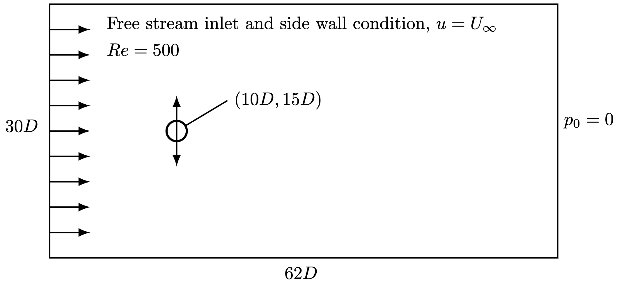
Fig. 2 A schematic of the domain showing the oscillating cylinder in a free-stream.

Problem description

The problem consists of a cylinder with diameter of \(D=10\) cm oscillaing in fluid flow subject to a free-stream velocity \(U_{\infty} = 1\) m/s, as shown in Fig. 2. For this simulation we also require the domain mesh as a separate file, which is located in the src/oasismove/mesh folder named cylinder.xdmf. A visualization of the triangulated mesh, and a zoomed in view on the cylinder is shown in Fig. 3.

Fig. 3 The computational domain for the oscillating cylinder in a free-stream. On the left, an overview of the domain, and on the right, a zoomed in view on the refinement around the cylinder.

Furthermore, the simulation is run for a Reynolds number equal to 500, which is adjustable in the problem file MovingCylinder.py . This will define the kinematic viscosity accordingly. Moreover, the oscillating movement is controlled by the amplitude ratio \(A_{ratio}\), the Strouhal number \(St\), and the frequency ratio \(F\). Based on these parameters, the frequency of the oscillations are defined as:

(4)\[ f = \frac{St U_{\infty}F}{D}.\]

Furthermore, the cylinder position followed a sinusoidal profile in the transverse direction to the flow:

(5)\[ \mathbf x( \mathbf X, t) = (0, A \sin (2 \pi f t )), \]

where \(A = A_{ratio}D\) is the amplitude.

Simulation in OasisMove

To run the oscillating cylinder problem for \(T=5\) seconds with default parameters in OasisMove you can run the following command:

$ oasismove NSfracStepMove problem=MovingCylinder Re=500 u_inf=1.0 F=1.0 T=5 mesh_path=src/oasismove/mesh/cylinder.xdmf

or without explicitly writing the default parameters:

$ oasismove NSfracStepMove problem=MovingCylinder mesh_path=src/oasismove/mesh/cylinder.xdmf

and the simulation will start. The default time step is relatively small, so the simulation might take some minutes before it is complete.

Results

When the simulation is finished, there will be a folder named results_moving_cylinder, which contains the velocity and pressure solution in .xdmf format, and the forces related to the simulation, including the drag (\(C_D\)) and lift ( \(C_L\)) coefficient defined as:

(6)\[ C_D = \frac{2 F_D}{\rho U_\infty^2 D}, \qquad C_L = \frac{2F_L}{\rho U_\infty^2 D}, \]

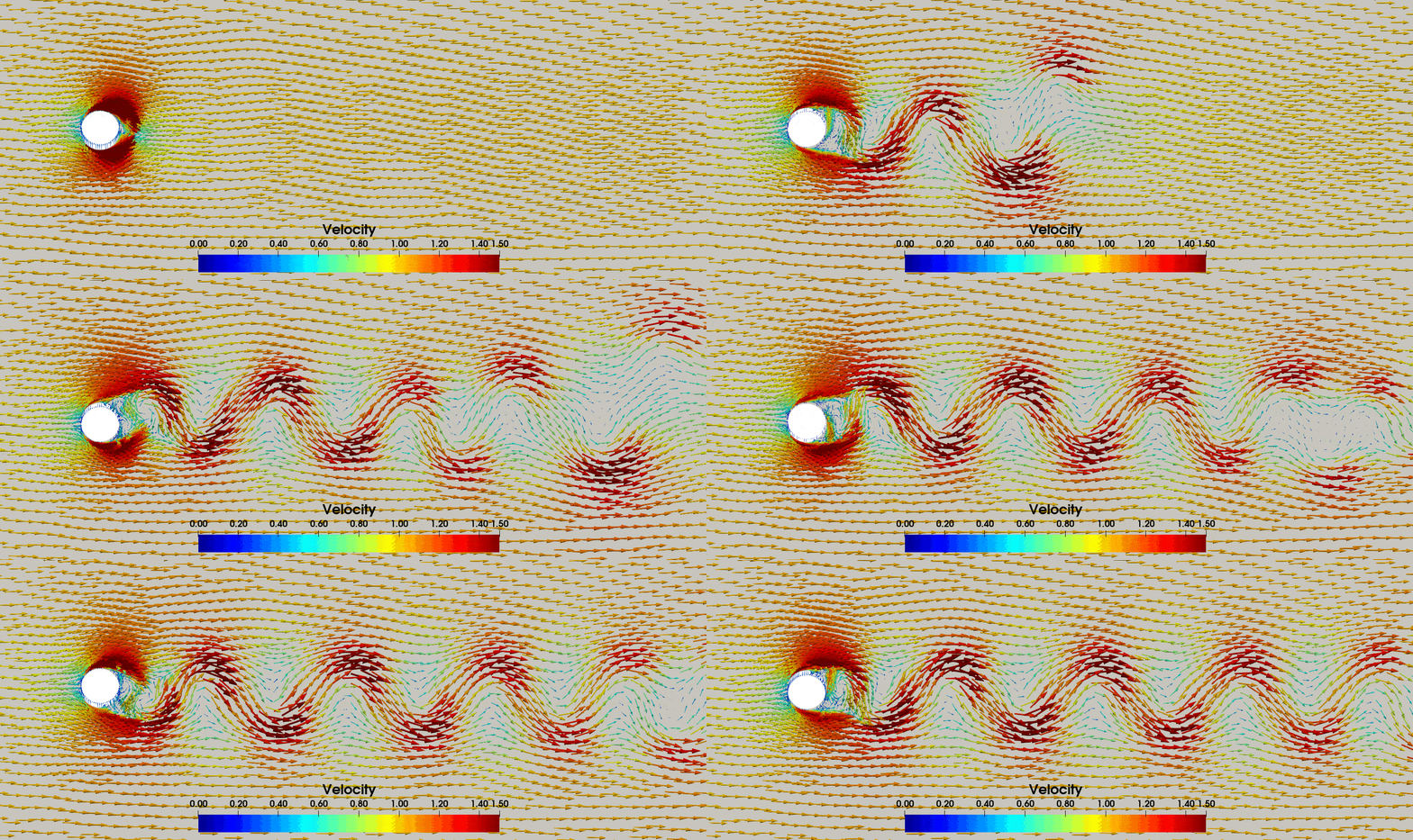
stored in the forces.txt file. In Fig. 4 we display the resulting velocity field, where we have added vectors scaled by the velocity magnitude. Furthermore, the values saved in the forces.txt file can be plotted to visualize the drag and lift coefficient over time, as visualized in Fig. 5.

Fig. 4 The velocity field for the oscillating cylinder in a free-stream, where the vector arrows have been scaled by the velocity magnitude.

Fig. 5 Drag (left) and lift (right) coefficient visualized over the simulation duration.

Adjusting the Reynolds number

The default Reynolds number (\(Re\)) for the oscillating cylinder problem is \(Re=500\). However, this can easily be adjusted by adding it as a command line argument. For instance, we can run a simulation with \(Re=100\) by running the following command:

$ oasismove NSfracStepMove problem=MovingCylinder Re=100 mesh_path=src/oasismove/mesh/cylinder.xdmf

As an example of adjusting the Reynolds number, we have run the simulation using \(Re=1, 20, 100,\) and \(500\). In Fig. 6, we have visualized the streamlines for the four velocity fields, with emphesis on the region in the wake of the cylinder.

Fig. 6 Streamlines for varying Reynolds numbers, raning from \(Re=1\) to \(Re=500\), colored by velocity magnitude.

Note that changing the Reynolds number will effectively adjust the kinematic viscosity \(\nu\), which is related to the Reynolds number by definition:

(7)\[ \text{Re } = \frac{U_{\infty} D}{\nu}\]

BH99

Hugh M Blackburn and Ron D Henderson. A study of two-dimensional flow past an oscillating cylinder. Journal of Fluid Mechanics, 385:255–286, 1999.