Cerebral aneurysm simulation#
A cerebral aneurysm is a pathological dilation of an artery in the brain. VaSP originated from research on cerebral aneurysms via high-fidelity fluid-structure interaction (FSI) simulations. For more context, please refer to the previous publications by Souche et al. [SVS22] and Bruneau et al. [BSVS23]. In this tutorial, we focus on meshing a cerebral aneurysm with interactive and local refinement and how to set up a high-fidelity FSI simulation under physiological conditions.
Meshing with interactive and local refinement#
Note
In this meshing section, we will use the data from AneuriskWeb. Specifiacally, we will use the geometry C0002 which is a 3D model of a cerebral aneurysm and can be downloaded from here.
In the previous tutorial, we used an objective method for determining the local mesh density, namely diameter-based meshing. In this tutorial, we will introduce a more interactive method for refining the mesh locally. This method is particularly useful when you want to refine the mesh in specific regions of the geometry, such as the aneurysm sac. To interactively refine the mesh, run:
vasp-generate-mesh -i C0002/surface/model.vtp -sch5 0.001 -st constant -m distancetospheres -mp 0 0.2 0.4 0.7 0 0.1 0.6 0.7 -fli 5 -flo 2
The flag -sch5 or (--scale-factor-h5) specifies the scaling factor from the original surface mesh to the volumetric mesh with .h5 extension. The flag -st constant (or --solid-thickness constant) specifies that the wall thickness of the mesh should be constant across the geometry. The flag -m distancetospheres (or --meshing-method distancetospheres) specifies the method for meshing the geometry. The flag -mp (or --meshing-parameters) specifies the parameters for the distance-to-sphere scaling function. When -m distancetospheres is selected, you must define multiple sets of four parameters for the distance-to-sphere scaling function: offset, scale, min, and max. --meshing-parameters 0 0.2 0.4 0.7 0 0.1 0.6 0.7 will run the function twice and the render window will pop up twice, where you can adjust the local mesh density interactively. The following gif shows an example of how to interactively refine the mesh:
Fig. 13 An interactive method for specifying local mesh refinement, using VMTK. Press d on the keyboard to display the distances to the sphere, which will define the local mesh density.#
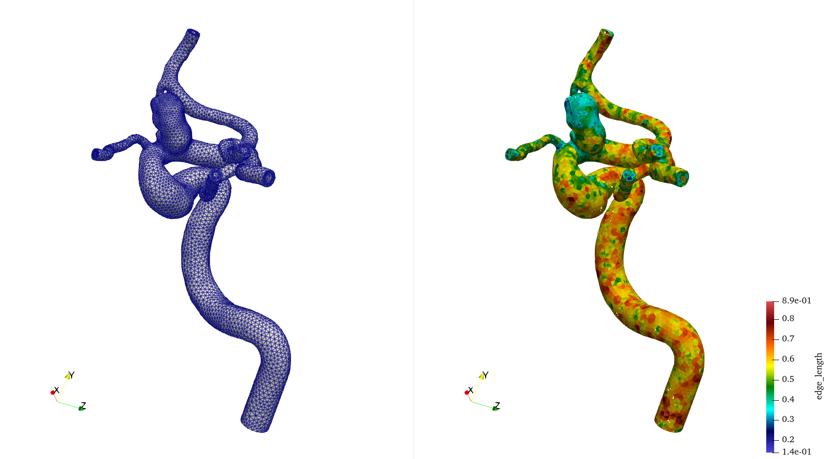
Fig. 14 The mesh of a cerebral aneurysm generated with local refinement as shown in the previous gif. On the left, you can see the mesh with edges. On the right, you can see the mesh color coded by the local mesh size.#
Running a FSI simulation#
Attention
To properly run high-fidelity FSI simulations of cerebral aneurysms, it is necessary to use a high-performance computing (HPC) cluster.
The simulation setup of a cerebral aneurysm is essentially the same as the offset stenosis case from the previous tutorial. Here, we focus on physiological boundary conditions and how they are defined in aneurysm.py.
Fluid boundary conditions#
First and foremost, we use Womersley velocity profile for the fluid inlet boundary condition where the mathematical expression is given by:
Here, \(r\) and \(t\) denote the cylindrical coordinates and time, respectively, and \(R\) is the radius of the inlet cross-section. \(J_{0}\) and \(J_{1}\) are Bessel functions of the first kind of orders 0 and 1, and \(\alpha_n\) is the Womersley number defined as \(\alpha_n = R\sqrt{n \omega/\nu}\) where \(\omega\) is the angular frequency of one cardiac cycle and \(\nu\) is the kinematic viscosity of the fluid. Finally, \(C_n\) are complex Fourier coefficients derived from the time-dependent flow rate as:
In VaSP, the coefficients \(C_n\) are obtained from the internal carotid arteries of older adults [HWX+10], located at src/vasp/simulations/FC_MCA10
In the aneurysm.py file, we define the Womersley velocity profile through VaMPy as follows:
from vampy.simulation.Womersley import make_womersley_bcs, compute_boundary_geometry_acrn
... # omitted code
def create_bcs(t, DVP, mesh, boundaries, mu_f,
               fsi_id, inlet_id, inlet_outlet_s_id,
               rigid_id, psi, F_solid_linear, p_deg, FC_file,
               Q_mean, P_FC_File, P_mean, T_Cycle, **namespace):

    # Load fourier coefficients for the velocity and scale by flow rate
    An, Bn = np.loadtxt(Path(__file__).parent / FC_file).T
    # Convert to complex fourier coefficients
    Cn = (An - Bn * 1j) * Q_mean
    _, tmp_center, tmp_radius, tmp_normal = compute_boundary_geometry_acrn(mesh, inlet_id, boundaries)

    # Create Womersley boundary condition at inlet
    tmp_element = DVP.sub(1).sub(0).ufl_element()
    inlet = make_womersley_bcs(T_Cycle, None, mu_f, tmp_center, tmp_radius, tmp_normal, tmp_element, Cn=Cn)
    # Initialize inlet expressions with initial time
    for uc in inlet:
        uc.set_t(t)

    # Create Boundary conditions for the velocity
    u_inlet = [DirichletBC(DVP.sub(1).sub(i), inlet[i], boundaries, inlet_id) for i in range(3)]
FC_file is the file containing the Fourier coefficients, Q_mean is the mean flow rate, and T_Cycle is the cardiac cycle period (mostly 0.951 s). The function compute_boundary_geometry_acrn computes the center, radius, and normal of the fluid inlet. The function make_womersley_bcs returns FEniCS Expression objects for the Womersley velocity profile, which are then used to define the fluid inlet boundary condition using DirichletBC.
Additionally, to avoid the sudden increase of flow at the beginning of the simulation, we use a ramp function to gradually increase the flow rate to the desired value. The following code shows how it is implemented in aneurysm.py:
def pre_solve(t, inlet, interface_pressure, **namespace):
    for uc in inlet:
        # Update the time variable used for the inlet boundary condition
        uc.set_t(t)

        # Multiply by cosine function to ramp up smoothly over time interval 0-250 ms
        if t < 0.25:
            uc.scale_value = -0.5 * np.cos(np.pi * t / 0.25) + 0.5
        else:
            uc.scale_value = 1.0
Fluid-solid interface boundary conditions#
Secondly, we also apply arterial pressure at the fluid-solid interface. The waveform is the same as the flow rate waveform, but the pressure is scaled to vary between 70 and 110 mmHg. This boundary condition is implemented weakly by modifying the FEniCS variational form as follows:
from vasp.simulations.simulation_common import InterfacePressure
... # omitted code
def create_bcs(t, DVP, mesh, boundaries, mu_f,
               fsi_id, inlet_id, inlet_outlet_s_id,
               rigid_id, psi, F_solid_linear, p_deg, FC_file,
               Q_mean, P_FC_File, P_mean, T_Cycle, **namespace):

    # Load Fourier coefficients for the pressure
    An_P, Bn_P = np.loadtxt(Path(__file__).parent / P_FC_File).T

    # Apply pulsatile pressure at the fsi interface by modifying the variational form
    n = FacetNormal(mesh)
    dSS = Measure("dS", domain=mesh, subdomain_data=boundaries)
    interface_pressure = InterfacePressure(t=0.0, t_ramp_start=0.0, t_ramp_end=0.2, An=An_P,
                                            Bn=Bn_P, period=T_Cycle, P_mean=P_mean, degree=p_deg)
    F_solid_linear += interface_pressure * inner(J_(d_["n"]("+")) * inv(F_(d_["n"]("+"))).T * n("+")) * dSS(fsi_id)
Here, P_FC_File is the file containing the Fourier coefficients for the pressure waveform, and P_mean is the mean pressure value. The InterfacePressure class is defined in VaSP and returns an floating value (Pa) for the pulsatile pressure waveform. The pressure is applied weakly to the fluid-solid interface by modifying the variational form F_solid_linear. Note that the normal vector n needs to be updated as the fluid-solid interface moves during the simulation. To do that, we use Nanson’s formula:
where \(F\) is the deformation gradient, \(J\) is the determinant of \(F\), and \(n^{'}\) is the updated normal vector.
Incorporating perivascular damping#
Finally, to incorporate viscoelastic damping from the perivascular environment, we use Robin boundary conditions at the solid outer wall, as introduced by Moireau et al. [MXA+12]. This has been already implemented in turtFSI and can be activated by setting the respective parameter as follows:
def set_problem_parameters(default_variables, **namespace):
    default_variables.update(dict(
    ... # omitted other parameters
    robin_bc=True,
    k_s=[1E5], # elastic coefficient [N*s/m^3]
    c_s=[10], # viscous coefficient [N*s/m^3]
    ds_s_id=[33] # surface ID for robin boundary condition
    ))
    return default_variables
Here, k_s and c_s are the elastic and viscous coefficients, respectively, and ds_s_id is the surface ID for the Robin boundary condition.
David A. Bruneau, David A. Steinman, and Kristian Valen-Sendstad. Understanding intracranial aneurysm sounds via high-fidelity fluid-structure-interaction modelling. Communications Medicine, 3(1):1–11, 2023. doi:10.1038/s43856-023-00396-5.
Yiemeng Hoi, Bruce A Wasserman, Yuanyuan J Xie, Samer S Najjar, Luigi Ferruci, Edward G Lakatta, Gary Gerstenblith, and David A Steinman. Characterization of volumetric flow rate waveforms at the carotid bifurcations of older adults. Physiological Measurement, 31(3):291–302, mar 2010. doi:10.1088/0967-3334/31/3/002.
P. Moireau, N. Xiao, M. Astorino, C. A. Figueroa, D. Chapelle, C. A. Taylor, and J. F. Gerbeau. External tissue support and fluid-structure simulation in blood flows. Biomechanics and Modeling in Mechanobiology, 11(1-2):1–18, 2012. doi:10.1007/s10237-011-0289-z.
Alban Souche and Kristian Valen-Sendstad. High-fidelity fluid structure interaction simulations of turbulent-like aneurysm flows reveals high-frequency narrowband wall vibrations: A stimulus of mechanobiological relevance? Journal of Biomechanics, 145:111369, dec 2022. doi:10.1016/j.jbiomech.2022.111369.