Running Fluid Structure Interaction (FSI) Simulations#
Simulations using turtleFSI#
VaSP uses turtleFSI for performing FSI simulations. In short, turtleFSI is a monolithic FSI solver built based on FEniCS. For the detailed usage of turtleFSI and tutorials, users are referred to the turtleFSI documentation. Here, we will introduce the very basic command for using turtleFSI and supporting functions that are specifically added for performing vascular FSI.
To run FSI simulations with turtleFSI, users typically need to create a problem file that contains information about input parameters and boundary conditions. How to create your own problem file is explained in details here. With the problem file and the mesh from pre-processing step in hand, you can now run FSI simulation with turtleFSI as follows:
turtleFSI -p name_of_the_problem_file (without .py)
It is also possible to run turtleFSI with Message Passing Interface (MPI) for possibly speeding up the simulation. To run turtleFSI with MPI, please use:
mpirun -np [number_of_cpu] -p name_of_the_problem_file (without .py)
turtleFSI also supports using config file for changing the parameter without modifying the original problem file. To run a problem file with config file, please use:
turtleFSI -p name_of_the_problem_file (without .py) -c path_to_config_file
An example of config file is located here.
For example, if the user want to run a problem file named my_problem.py with config file my_config.config using 4 processors, the command should be:
mpirun -np 4 turtleFSI -p my_problem -c my_config.config
In this case, it is assumed that my_problem.py and my_config.config are located in the same folder as the current working directory.
Monitoring tool during the simulation#
Due to the nature of vascular FSI simulations, it is usually the case that the simulation needs to be run on the supercomputer with many CPUs where the total simulation time may exceed one day. In such a case, it is crucial to monitor the progress of your simulations and check if the simulations are going as you wish. For that purpose, vasp-log-plotter can be used to plot the relevant quantities based on the log file generated during the run.
Since the plot is generated based on the log file, users must use functions from vasp.simulations.simulation_common to print out the information in the log file. Particularly, functions such as load_probe_points,
print_probe_points, calculate_and_print_flow_properties are important. Example problem files located under src/vasp/simulations illustrates how to use those functions inside the problem files.
Quantities that can be plotted are as follows:
- cpu time per time-step against simulation time
- number of newton iterations to converge to the specified tolerance (absolute & relative)
- velocity and pressure magnitude at probe points in fluid domain over time
- displacement magnitude at probe points in solid domain over time
- flow rate at the inlet
- maximum, minimum, and average velocity in the entire domain
- maximum, minimum, and average CFL number in the entire domain
- maximum, minimum, and average Reynolds number in the entire domain
To get a complete list of the parameters, please run:
vasp-log-plotter --help
Fig. 4 is an example of the plot showing CPU time per time-step and CFL number.
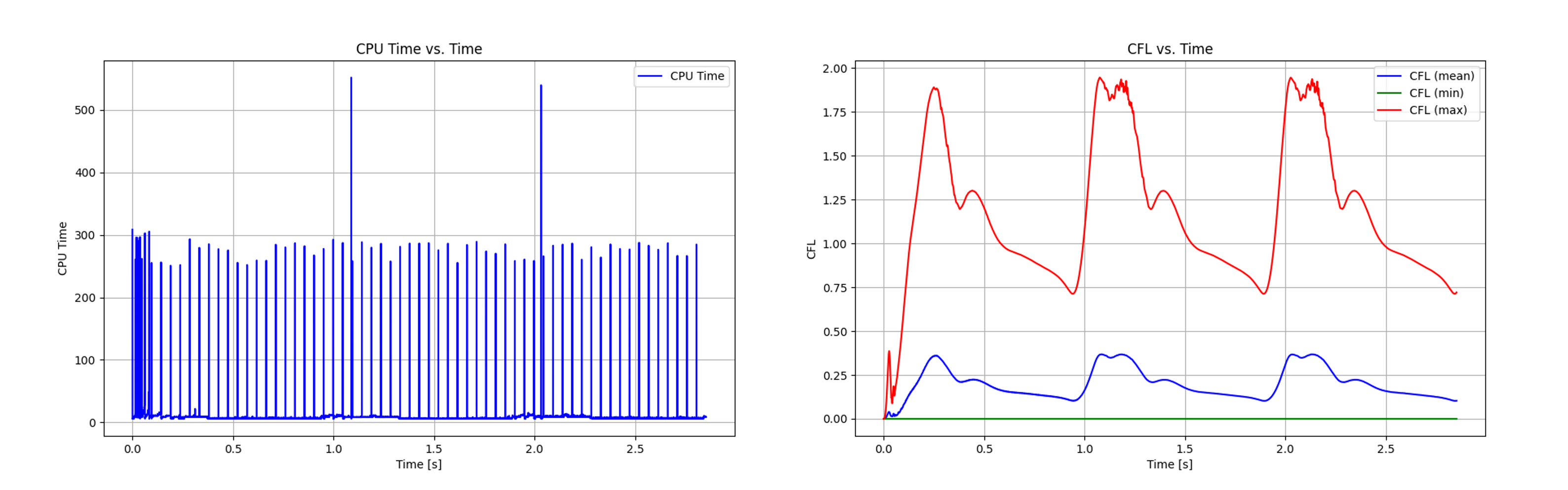
Fig. 4 An example of plots generated by vasp-log-plotter function#