Offset stenosis simulation#
As a first tutorial, we will illustrate major functionalities of VaSP with a non-axisymmetric stenosis model. This stenosis model is a synthetic geometry that can be described analytically and has been long used within fluid mechanics research [VFF07]. Due to the stenotic region with sudden area reduction, the flow becomes turbulent quickly without complex geometry or high Reynolds number. Additionally, eccentricity ensures that the simulation is deterministic, avoiding uncertainty associated with the symmetric geometry. Those features enable us to quickly develop and test the functionalities with reasonable computing time.
Mesh generation#
Note
An input mesh, offset_stenosis.stl, can be downloaded here.
There are couple of methods for determining the size of each tetrahedral cell, but VaSP uses centerline diameter by default. Details on different meshing strategy can be found here.
With that in mind, one can generate the mesh as follows:
vasp-generate-mesh -i offset_stenosis.stl -f True -fli 0 -flo 4 -c 3.8 -nbf 1 -nbs 1 -sch5 0.001
Here, -f is a boolean argument determining whether to add flow extensions or not, as explained in here. In this case, -flo 0 indicates no flow extension at the inlet, but -flo 4 will add flow extensions at the outlet with length equal to four times the length of radius of the outlet. -c is a coarsing factor determining the density of the mesh, where c > 1 will corasen the mesh. -nbf and -nbs are the number of sublayers for fluid boundary layer and solid domain, respectively. In this offset stenosis problem, we only use one layer as solid to speed up the computation.The last flag -sch5 will scale the mesh from [mm] to [m].
An example of the log during the pre-processing is:
Click to expand log output
Failed to import probe.probe11
Error message: Couldn't find a file matching the module name: probe.probe11  (opt_in = False)
Neither oasis nor oasismove is installed. Exiting simulation..
Neither oasis nor oasismove is installed. Exiting simulation..
WARNING: OasisMove is not installed, running moving domain CFD is not available
WARNING: OasisMove is not installed, running moving domain simulations (MovingAtrium) is not available
— Working on case: offset_stenosis
— Load model file

— Surface overview:
Total number of triangles: 14993.
Total number of points: 7583.
— Check the surface.
Found 0 NaN cells.
— Cleaning the surface.
Done.
— Check the surface.
Found 0 NaN cells.

— Get centerlines
Cleaning surface.
Triangulating surface.
Computing centerlines.
Computing centerlines…
— No smoothing of surface
— Adding flow extensions
— Compute the model centerlines with flow extension.
Cleaning surface.
Triangulating surface.
Computing centerlines.
Computing centerlines…— Computing distance to sphere
— Generating FSI mesh
Not capping surface
Remeshing surface
Iteration 1/10
Iteration 2/10
Iteration 3/10
Iteration 4/10
Iteration 5/10
Iteration 6/10
Iteration 7/10
Iteration 8/10
Iteration 9/10
Iteration 10/10
Final mesh improvement
Computing projection
Generating boundary layer fluid
Generating boundary layer solid
Capping inner surface
Remeshing endcaps
Iteration 1/10
Iteration 2/10
Iteration 3/10
Iteration 4/10
Iteration 5/10
Iteration 6/10
Iteration 7/10
Iteration 8/10
Iteration 9/10
Iteration 10/10
Final mesh improvement
Computing sizing function
Generating volume mesh
TetGen command line options: pq1.414000q10.000000q165.000000YsT1.000000e-08zQm
Assembling fluid mesh
Assembling final FSI mesh
— Writing Dolfin file
— Converting XML mesh to HDF5
— Flattening the inlet/outlet if needed
Surface with ID 2 is not flat: Standard deviation of facet unitnormals is 0.031194747575524318, greater than threshold of 0.001
Moving nodes into a flat plane
Surface with ID 3 is not flat: Standard deviation of facet unitnormals is 0.014826901671377794, greater than threshold of 0.001
Moving nodes into a flat plane
Changes made to the mesh file
— Evaluating edge length
=== Mesh information ===
X range: -9.53805 to 24.8625 (delta: 34.4006)
Y range: -3.45556 to 3.4564 (delta: 6.9120)
Z range: -3.45595 to 3.45649 (delta: 6.9124)
Number of cells: 20829
Number of cells per processor: 20829
Number of edges: 0
Number of faces: 42581
Number of facets: 42581
Number of vertices: 3890
Volume: 1166.8263
Number of cells per volume: 17.8510
— Saving probes points in: offset_stenosis_probe_point.json
Your folder with input mesh should now look like:
Folder
├── commands_20250114132437.txt
├── offset_stenosis.h5
├── offset_stenosis.stl
├── offset_stenosis.vtu
├── offset_stenosis.xml.gz
├── offset_stenosis_boundaries.pvd
├── offset_stenosis_boundaries000000.vtu
├── offset_stenosis_domains.pvd
├── offset_stenosis_domains000000.vtu
├── offset_stenosis_edge_length.h5
├── offset_stenosis_edge_length.xdmf
├── offset_stenosis_info.json
└── offset_stenosis_probe_point.json
Finally, to generate solid probes, please run:
vasp-generate-solid-probe --mesh-path offset_stenosis.h5 --fsi-region -0.0002 0.016 -0.0035 0.0035 -0.0035 0.0035
Fig. 7 shows an example of the volumetric mesh.
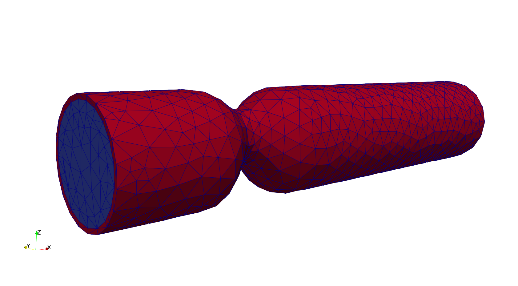
Fig. 7 Volumetric mesh of offset stenosis with solid (red) and fluid (blue) regions.#
FSI simulations#
Note
An input mesh for FSI simulation, offset_stenosis.h5, can be downloaded here. Additionally, fluid and solid probe points are also required to run this problem and can be downloaded here and here.
The next step is to run FSI simulation using turtleFSI. First, make sure to move to the folder where offset_stenosis.py is located, i.e. src/vasp/simulations/. Then, one can simply run
turtleFSI -p offset_stenosis --mesh_path=/path/to/your_folder/offset_stenosis.h5
where --mesh-path is the path to the volumetric mesh generated from the pre-processing. While this problem can be executed on a normal laptop, it may be quite slow. As such, it is highly recommended to speed up the computation by using MPI. For example, one can use eight processors as:
mpirun -np 8 turtleFSI -p offset_stenosis --mesh_path=/path/to/your_folder/offset_stenosis.h5
to speed up the simulation.
During the FSI simulation, turtleFSI will print out some information that are useful for monitoring the progress. A simplified example of such a log is
Flow Properties:
  Flow Rate at Inlet: 1.9492469835105836e-06
  Velocity (mean, min, max): 0.05444848866112857, 4.11345811806542e-16, 0.49485295630442205
  CFL (mean, min, max): 0.2379617502537257, 1.797746305617944e-15, 0.9627060455857645
  Reynolds Numbers (mean, min, max): 226.8227703002397, 1.7135938733956218e-12, 1061.4698626220043
Solved for timestep 122, t = 0.1220 in 7.4 s
ramp_factor = 0.6767374218896292
Instantaneous normal stress prescribed at the FSI interface 9648.21114507385 Pa
Newton iteration 0: r (atol) = 3.712e-02 (tol = 1.000e-06), r (rel) = 1.988e-02 (tol = 1.000e-06)
Newton iteration 1: r (atol) = 5.473e-05 (tol = 1.000e-06), r (rel) = 1.914e-02 (tol = 1.000e-06)
Newton iteration 2: r (atol) = 4.711e-06 (tol = 1.000e-06), r (rel) = 1.943e-04 (tol = 1.000e-06)
Probe Point 1: Velocity: (0.09891215934965708, 0.0003292221793639628, 0.009674117733206467) | Pressure: 93.38433393779773
Probe Point 1: Displacement: (-3.304118240759384e-05, 0.00018922478784845321, 0.00017120957053687062)
Results of the simulation are saved in a folder offset_stenosis_results with the following structure:
offset_stenosis_results/1
├── Checkpoint
│   ├── checkpoint_d1.h5
│   ├── checkpoint_d1.xdmf
│   ├── checkpoint_p1.h5
│   ├── checkpoint_p1.xdmf
│   ├── checkpoint_v1.h5
│   ├── checkpoint_v1.xdmf
│   └── default_variables.json
├── Mesh
│   └── mesh.h5
└── Visualization
    ├── displacement.h5
    ├── displacement.xdmf
    ├── pressure.h5
    ├── pressure.xdmf
    ├── velocity.h5
    └── velocity.xdmf
Post-processing#
Post-processing Mesh#
The first step of post-processing is to refine mesh as we used save_deg=2, but this can be skipped in case you run the simulation with save_deg=1. To refine the mesh, run:
vasp-refine-mesh --folder offset_stenosis_results/1
where an example log is:
Click to expand log output
--- Refined mesh saved to: offset_stenosis_results/1/Mesh/mesh_refined.h5

--- Correcting node numbering in refined mesh

--- Node numbering is incorrect between the refined mesh and the output velocity.h5 file

--- Sorting node coordinates

x coordinate is not unique and sort based on x, y, and z coordinates

--- Correcting node numbering of the topology array in the refined mesh

--- Correcting node numbering of the boundary topology array in the refined mesh

--- Correcting boundary values in the refined mesh

--- Saving the corrected node numbering to the refined mesh

The node numbering in the refined mesh has been corrected to match the output velocity.h5 file
Note
At a later stage in the post-processing, we will use refined mesh to extract domain specific variables, such as fluid velocity, from velocity.h5. For that to work properly, we perform sorting of the node numbering as indicate in the log.
The next step is to separate the mesh into fluid and solid only meshes by executing:
vasp-separate-mesh --folder offset_stenosis_results/1
with an example log:
Click to expand log output
--- Separating fluid and solid domains using domain IDs

--- Fluid domain ID: [1, 1001] and Solid domain ID: 2

--- Saving fluid domain to offset_stenosis_results/1/Mesh/mesh_fluid.h5

--- Saving solid domain to offset_stenosis_results/1/Mesh/mesh_solid.h5

--- Done separating domains

--- fluid topology does not need to be fixed

--- Saving the fixed mesh file

--- Fixing topology of solid domain

--- Saving the fixed mesh file

--- Refined mesh exists, separating domains for refined mesh

--- Saving fluid domain to offset_stenosis_results/1/Mesh/mesh_refined_fluid.h5

--- Saving solid domain to offset_stenosis_results/1/Mesh/mesh_refined_solid.h5

--- Done separating domains

--- Fixing topology of fluid domain

--- Saving the fixed mesh file

--- Fixing topology of solid domain

--- Saving the fixed mesh file
Post-processing FEniCS#
In this section, we will go through how to separate fluid velocity and solid displacement from the original visualization files. This procedure will enable efficient computation of hemodynamics and stress/strain at a later stage.
First, you need to create FEniCS-compatible files as original visualization files from turtleFSI can not be re-read by FEniCS. To do so, run:
vasp-create-hdf5 --folder offset_stenosis_results/1
which creates u.h5 and d_solid.h5 under newly created folder Visualization_separate_domain.
To visualize those separated variables, you can run
vasp-create-separate-domain-viz --folder offset_stenosis_results/1
Fig. 8 is an visualization of domain specific visualization.
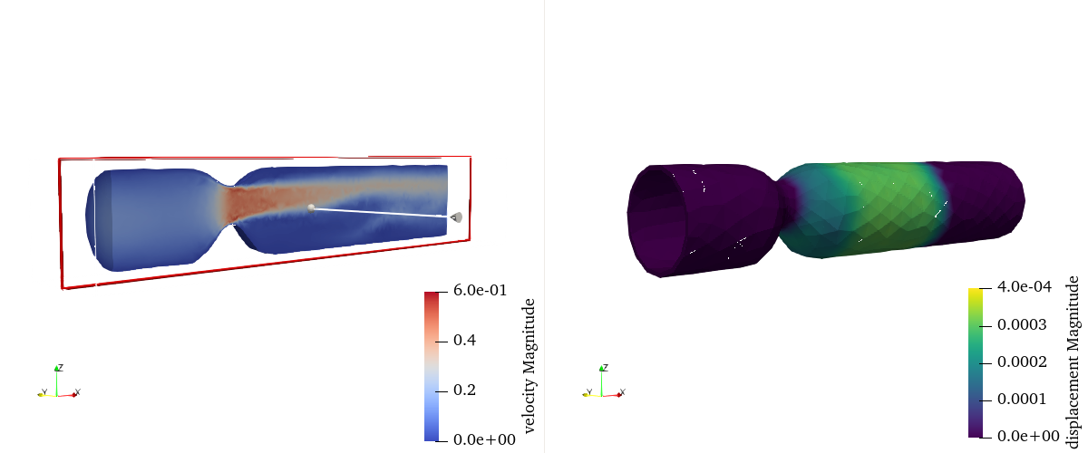
Fig. 8 Fluid velocity (left) and solid displacement (right)#
Finally, hemodynamics and stress/strain can be computed, independently and simultaneously, as:
vasp-compute-hemo --folder offset_stenosis_results/1
and
vasp-compute-stress --folder offset_stenosis_results/1
Fig. 9 and Fig. 10, respectively, show computed hemodynamics and stress/strain.
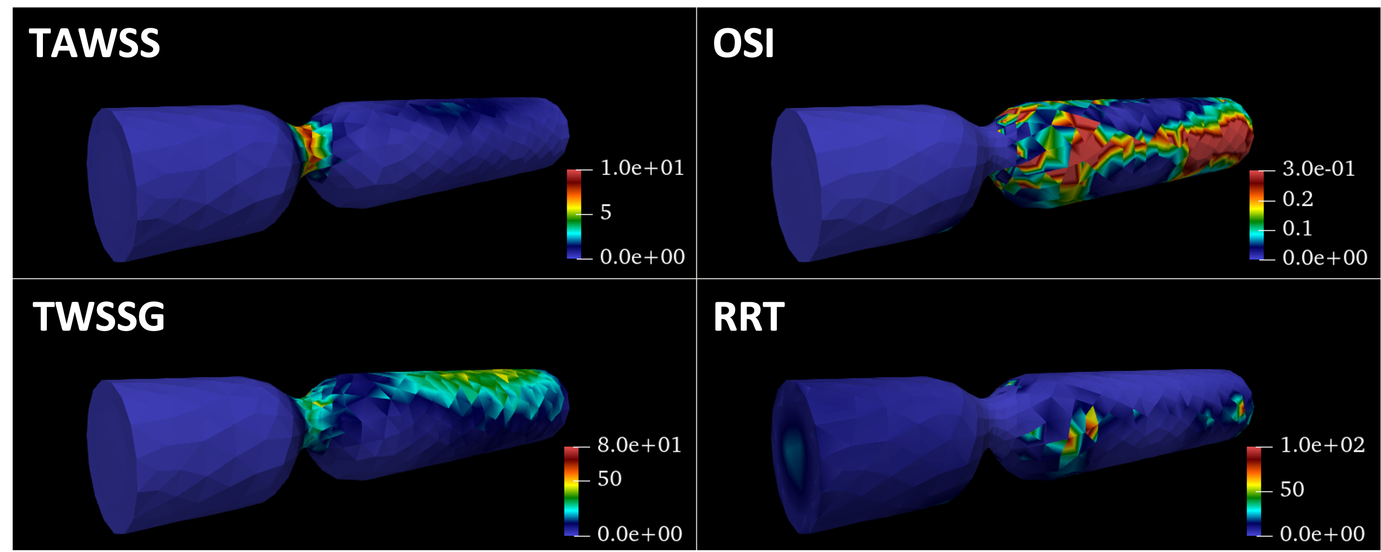
Fig. 9 Hemodynamic indices computed based on fluid velocity#
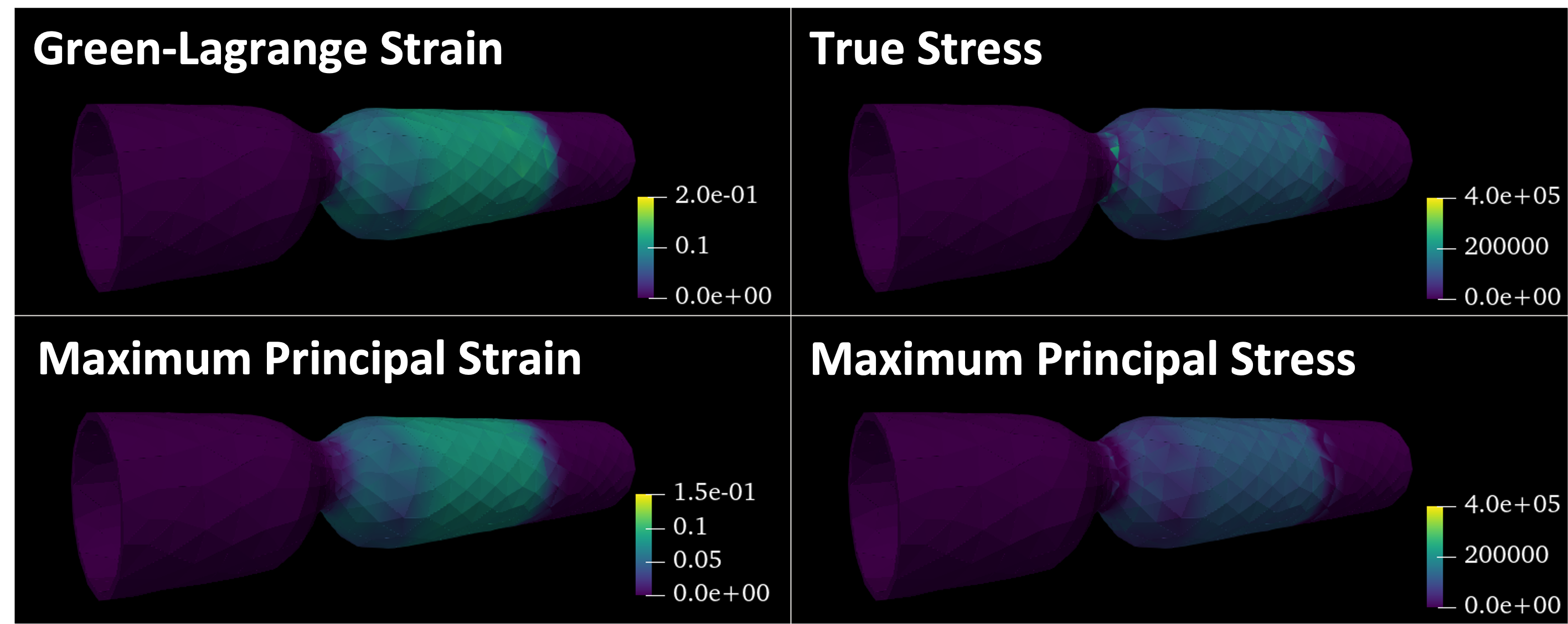
Fig. 10 Solid stress and strain computed based on solid displacement#
Post-processing h5py#
Attention
While this section comes after post-processing fenics, all the post-processing in this section can be performed as long as you have meshes from the post-processing mesh.
We first start by generating spectrograms, which represent the evolution of frequency over time. To do so, run:
vasp-create-spectrograms-chromagrams --folder offset_stenosis_results/1 -q d --component all --start-time 0.951 --end-time 1.902 --ylim 500
Here, -q indicates the quantity of interest, namely displacement (d), velocity (v), or pressure (p). The second flag --component specifies which directional component to use, where all means that we use all x, y, and z components to generate spectrograms. --start-time/end-time and --ylim are used to specify the time-window, i.e. x-axis, and maximum frequency, i.e. y-axis, of the resulting spectrograms. In this example, we focus on the second cardiac cycle (0.951 ~ 1.902 s) and up to 500 Hz. Fig. 11 is an example of the figure you get as a result. For detailed explanation of chromagram and spectral bandness index, please refer to MacDonald et al. [MNTS22]
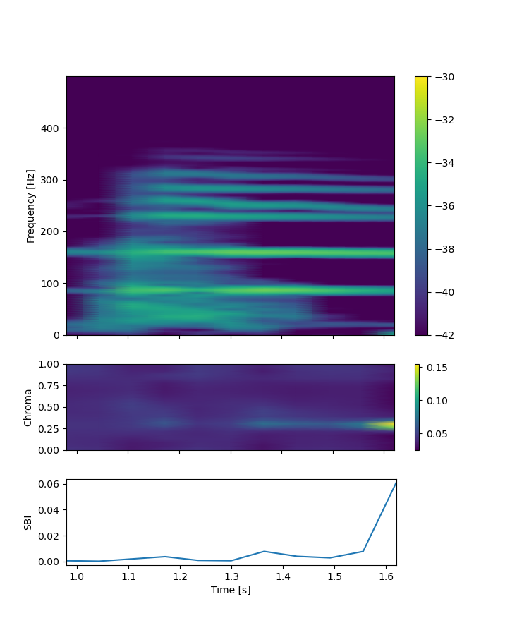
Fig. 11 Displacement spectrogram (top), chromagram (middle), and spectral bandness index (SBI, bottom)#
Now, from the spectogram, it is quite clear that there are some concentration of the frequency contents, as evident from narrow frequency bands. Physically, those frequency are associated with the specific directional motion of the wall, called mode shapes. To extract and visualize such motions, you can use vasp-create-hi-pass-viz command. For example, two distinct modes (70 ~ 90 Hz and 150 ~ 170 Hz) can be extracted by running the following command:
vasp-create-hi-pass-viz --folder offset_stenosis_results/1 -q d --start-time 0.951 --end-time 1.902 --bands 70 90
and
vasp-create-hi-pass-viz --folder offset_stenosis_results/1 -q d --start-time 0.951 --end-time 1.902 --bands 150 170
Those two modes correspond to the specific motion of the stenosis wall, as shown in Fig. 12.
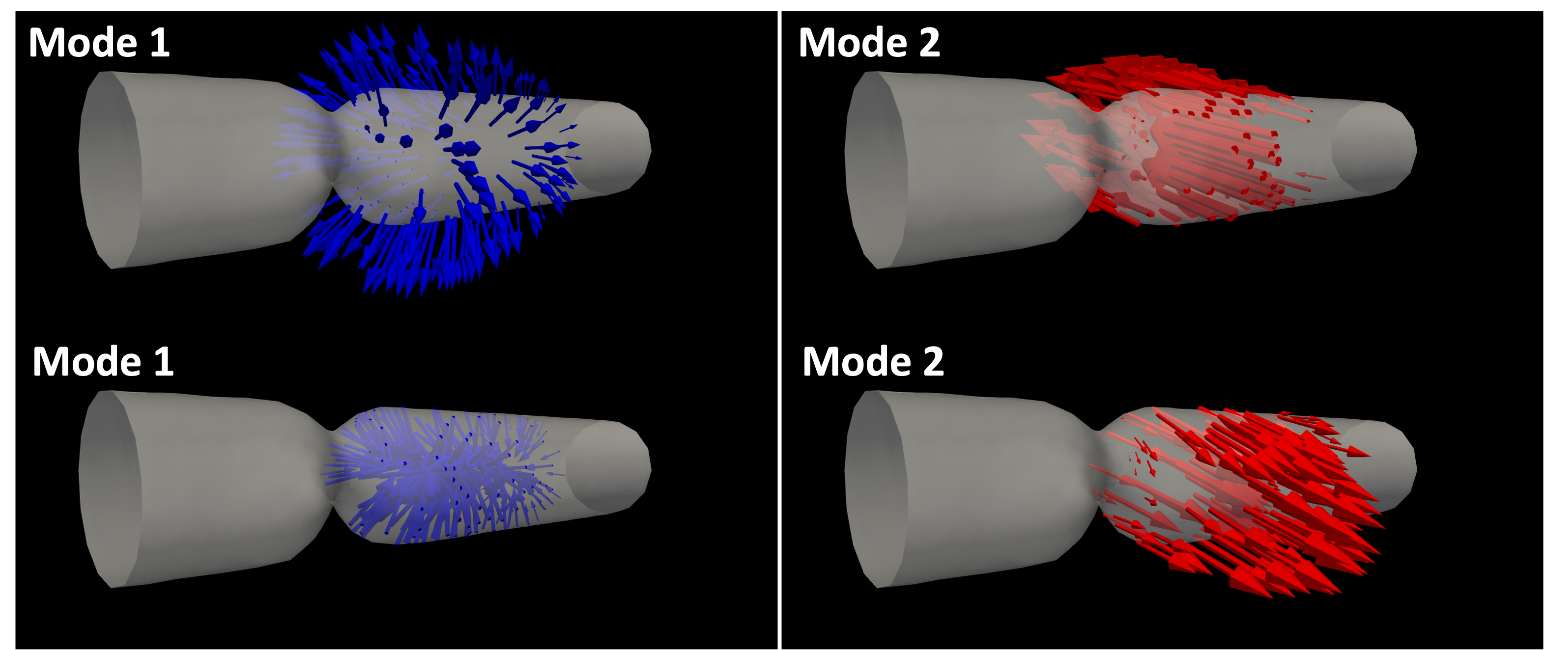
Fig. 12 Mode shapes of stenosis with expansion/contraction (mode1) and left/right (mode2) motions#
Daniel E. MacDonald, Mehdi Najafi, Lucas Temor, and David A. Steinman. Spectral Bandedness in High-Fidelity Computational Fluid Dynamics Predicts Rupture Status in Intracranial Aneurysms. Journal of Biomechanical Engineering, 2022. doi:10.1115/1.4053403.
Sonu S. Varghese, Steven H. Frankel, and Paul F. Fischer. Direct numerical simulation of stenotic flows. Part 1. Steady flow. Journal of Fluid Mechanics, 582:253–280, 2007. doi:10.1017/S0022112007005848.