Arteriovenous Fistulas (AVF) simulation

An arteriovenous fistula (AVF) is a vascular abnormality that forms between an artery and a vein. Since an AVF involves two distinct types of vascular tissues, it is necessary to generate a mesh with variable wall thickness and assign unique domain markers for the artery and vein. In this example, we focus on advanced meshing techniques that incorporate multiple solid domains. The methodology is originally developed in the previous publications by Bozetto et al. [BRVS24] and Soliveri et al. [SBR+24]. For detailed descriptions of the methodology, please refer to the original publications.

Meshing an AVF with variable wall thickness

Note

An input surface mesh can be downloaded here.

To generate a mesh with different wall thickness and domain markers between artery and vein, run:

vasp-generate-mesh -i avf.stl -st variable -stp 0 0.05 0.15 0.3 -eb -c 2.0 -m diameter -f False 

The first flag -st variable (or --solid-thickness variable) specifies that the wall thickness of the mesh should vary across the geometry. This is particularly useful for modeling physiological structures where different regions have distinct mechanical properties or geometrical features, such as arteries and veins. The second flag -stp (or --solid-thickness-parameters) is used to specify the parameters for the variable wall thickness. When -st variable is selected, you must define four parameters for the distance-to-sphere scaling function: offset, scale, min, and max. These parameters control how the wall thickness changes across the geometry. With this option, a render window will pop up, where you can specify the wall thickness interactively as follows:

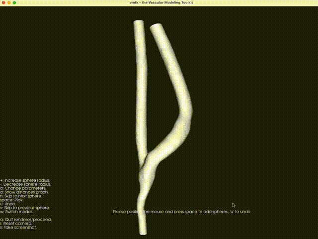
Fig. 14 An interactive method for specifying variable wall thickness, using VMTK. Press d on the keyboard to display the distances to the sphere, which will define the local wall thickness. In this case, the red regions will have a wall thickness of 0.15, while the blue regions will have a wall thickness of 0.3.

The third option -eb (or --extract-branch) option enables the extraction of specific branches from the mesh, such as the artery or vein in an AVF. When this option is enabled, VaSP assigns a unique solid mesh ID to the extracted branch, with an optional ID offset, controlled by --branch-ids-offset. This offset allows for the modification of the original solid ID number. For instance, if the original ID for a solid is 2 and the offset is set to 1000, the extracted branch will be assigned a new solid ID of 1002. This feature is particularly useful when you want to separately treat specific branches, like the artery and vein, with different wall properties. Again, with this option enabled, a render window will pop up, allowing you to specify the branch interactively.

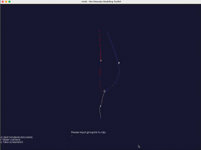
Fig. 15 An interactive method for extracting branches, using VMTK. Type the branch ID to extract the corresponding branch. In this case, the vein is extracted with a branch ID of 0.

In case you already know the branch IDs, you can specify them directly using the --branch-group-ids option, avoiding the interactive selection.

Finally, Fig. 16 shows the generated computational domains for the AVF geometry. The artery and vein are assigned different solid IDs with different wall thicknesses.

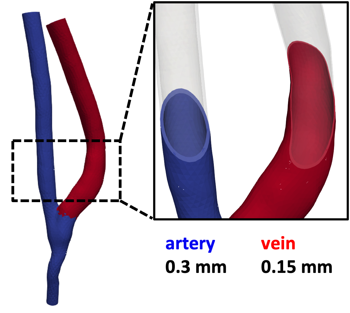
Fig. 16 The artery and vein are assigned different solid IDs with different wall thicknesses.

Running a FSI simulation

The main difference of running a FSI simulation with an AVF model compared to a cerebral aneurysm model is the presence of multiple solid domains. This difference is, indeed, reflected in the simulation setup. In avf.py, we specify the solid IDs for the artery and vein, as well as the corresponding wall properties. The following code snippet shows how to define the solid IDs and wall properties for the AVF model:

def set_problem_parameters(default_variables, **namespace):

    default_variables.update(dict(
        ... # other omitted parameters
        dx_s_id=[2, 1002],  # ID of marker in the solid domain
        solid_properties=[{"dx_s_id": 2, "material_model": "MooneyRivlin", "rho_s": 1.0E3, "mu_s": mu_s_val_artery,
                           "lambda_s": lambda_s_val_artery, "C01": 0.03e6, "C10": 0.0, "C11": 2.2e6},
                          {"dx_s_id": 1002, "material_model": "MooneyRivlin", "rho_s": 1.0E3, "mu_s": mu_s_val_vein,
                           "lambda_s": lambda_s_val_vein, "C01": 0.003e6, "C10": 0.0, "C11": 0.538e6}],
        ... # other omitted parameters
    ))

Moreover, we use patient-specific boundary conditions for the AVF model. The following code snippet shows how to define the boundary conditions for the AVF model:

def create_bcs(DVP, mesh, boundaries, T, dt, fsi_id, inlet_id1, inlet_id2, rigid_id, psi, F_solid_linear,
               vel_t_ramp, p_t_ramp_start, p_t_ramp_end, p_deg, v_deg, patient_data_path, **namespace):
    # read patient-specific data
    patient_data = np.loadtxt(patient_data_path, skiprows=1, delimiter=",", usecols=(0, 1, 2))
    v_PA = patient_data[:, 0]
    v_DA = patient_data[:, 1]
    PV = patient_data[:, 2]

    len_v = len(v_PA)
    t_v = np.arange(len(v_PA))
    num_t = int(T / dt)  # 30.000 timesteps = 3s (T) / 0.0001s (dt)
    tnew = np.linspace(0, len_v, num=num_t)

    interp_DA = np.array(np.interp(tnew, t_v, v_DA))
    interp_PA = np.array(np.interp(tnew, t_v, v_PA))
    # pressure interpolation (velocity and pressure waveforms must be syncronized)
    interp_P = np.array(np.interp(tnew, t_v, PV))

In this code snippet, patient-specific boundary conditions are defined by interpolating measured data to match the simulation’s temporal resolution. The patient data is read from a CSV file, which extracts the velocity values for the proximal artery (v_PA), distal artery (v_DA), and the pressure values (PV). The time indices for the original dataset are then generated as t_v.

The simulation is run over a specified number of timesteps, calculated as num_t, which represents the total time (T) divided by the time increment (dt). To align the patient-specific data with the simulation’s temporal grid, a new array of time points (tnew) is created using np.linspace.

Finally, interpolation is performed for each dataset (v_PA, v_DA, and PV) using np.interp. This ensures that the velocity and pressure waveforms are synchronized with the simulation’s temporal resolution, enabling accurate application of boundary conditions in the AVF model.

[BRVS24]

Michela Bozzetto, Andrea Remuzzi, and Kristian Valen-Sendstad. Flow-induced high frequency vascular wall vibrations in an arteriovenous fistula: a specific stimulus for stenosis development? Physical and Engineering Sciences in Medicine, 47(1):187–197, 2024. doi:10.1007/s13246-023-01355-z.

[SBR+24]

Luca Soliveri, David Bruneau, Johannes Ring, Michela Bozzetto, Andrea Remuzzi, and Kristian Valen-Sendstad. Toward a physiological model of vascular wall vibrations in the arteriovenous fistula. Biomechanics and Modeling in Mechanobiology, 2024. doi:10.1007/s10237-024-01865-z.