Moving domain simulation of the left atrium

Moving domain simulation of the left atrium#

The third tutorial considers a moving domain CFD simulation in a simplified left atrium geometry. This hand-crafted geometry, named model.vtp, can be found in the models/moving_atrium directory and was designed by the VaMPy authors using the MeshMixer software. This tutorial aims to showcase VaMPy’s versatility, highlighting its capabilities beyond rigid wall simulations, particularly in the context of atrial simulations. Additionally, the tutorial introduces the concept of blood residence time (\(T_R\)) – a metric that captures blood flow stasis by solving a scalar transport equation.

Moving domain meshing of the left atrium#

The morphology of the simplified left atrium is depicted on the left side of Fig. 22. It features four pulmonary veins and a pouch-like structure representing the left atrial appendage. The left atrial appendage is particularly prone to blood clot formation, making it a significant region of interest within the left atrium. However, this tutorial focuses on showcasing the moving domain capabilities of VaMPy/OasisMove, so mesh refinement will not be discussed.

To perform moving domain meshing for this model, execute the command below:

$ vampy-mesh --moving-mesh -i models/moving_atrium/model.vtp -m constant -el 1.3 -fli 2 -flo 1.5 -at 

In this command, the -fli and -flo flags determine the length of the flow extensions at the inlets and outlet, respectively, and the -at flag is used to notify the pipeline that an atrium model is being meshed.

Upon successful execution, the meshing command will generate the standard output files. Additionally, it will produce the displacement matrix, stored in model_points.np, and the deformed surfaces with flow extensions in model_extended . The latter is illustrated in the middle figure of Fig. 22. The final volumetric mesh, inclusive of four boundary layers, is displayed on the right side of Fig. 22.

_images/simpleatrium.gif — Fig. 22 From left to right: the surface model used in this tutorial, the deformed model with flow extensions, and the resulting volumetric mesh based on the provided meshing parameters.#

The displacement field and `model_points.np`#

The model_points.np file introduces a new input for the CFD simulation, describing the displacement field of each surface point. Each point within model_points.np is accomponied by its discrete displacement over a full cycle. For moving domain simulations driven by image-based motion, OasisMove utilizes this displacement field to define the wall boundary conditions. The process within OasisMove is as follows:

Load displacement matrix: OasisMove identifies and loads the model_points.np file, storing the matrix in the points variable.
Spline interpolation: Using SciPy’s splrep method, spline interpolation is executed for each point, ensuring a continuous description of the deformation over one cycle (see the left-hand side of Fig. 23).
Mesh velocity computation: The first-order derivative of the spline is computed by OasisMove. This derivative represents the mesh velocity and is set as the wall boundary condition (see the right-hand side of Fig. 23).

To exemplify, we may consider the deformation field of the demo model located in the moving_atrium directory. Focusing on the surface point at index 1, the displacement curve, its spline-interpolated counterpart, and the mesh velocity for the \(x\)-component are illustrated in Fig. 23.

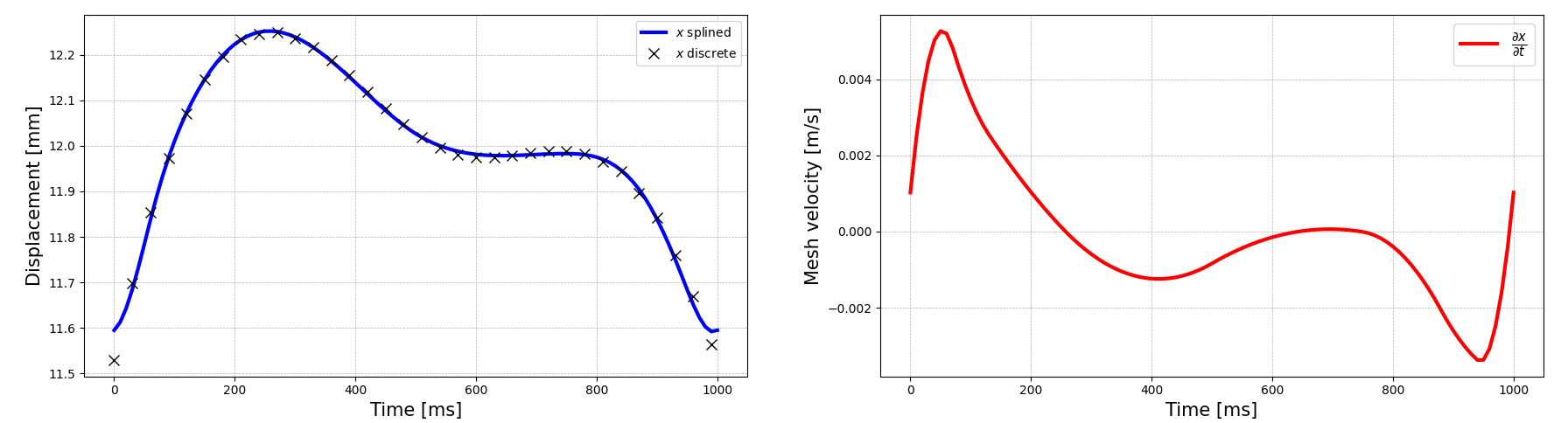
_images/spline.png — Fig. 23 On the left: the discrete displacement profile (x) for the surface point at index 1, together with its spline representation (blue curve). On the right: the first-order derivative, denoting the mesh velocity for that specific point.#

Quantifying blood residence time#

In the majority of patients with atrial fibrillation, there’s a risk of blood clot formation in the left atrial appendage. To further investigate this phenomenon using CFD simulations, it’s essential to assess the duration a blood particle remains within the left atrium and its appendage. This duration can be quantified by a scalar metric termed the blood residence time, \(T_R\).

The blood residence time, \(T_R\), is determined throughout the computational domain by solving a forced passive scalar equation, as formulated by Rossini et al.[RMLV+16]:

(1)#\[\frac{\partial T_R}{\partial t} + \mathbf u \cdot \nabla T_R = 1,\]

At the onset of the simulation, \(T_R\) is initialized to zero everywhere in the domain, including at the pulmonary veins as a boundary condition. Within OasisMove, Equation (1) is simulteneously solved as the Navier-Stokes equations, and incorperates a SUPG stabilization term to counteract the inherent instability of a purely advective transport equation.

Moving domain CFD simulation#

With the generated mesh, standard CFD input files, and the displacement field from model_points.np, we can start the moving domain CFD simulation. It’s important to note that such simulations are exclusively supported by OasisMove. The specifics of our CFD problem are outlined in the MovingAtrium.py file, found in the simulation directory. The inlet boundary conditions are defined by the normalized flow rate values located in the PV_values file, and are adjusted by the model’s mean flow rate. Meanwhile, the outlet is set with a zero-pressure boundary condition, and the wall boundary conditions are determined using the displacement field from model_points.np.

To execute a moving domain CFD simulation of the left atrium model over four cardiac cycles, navigate to the src/vampy/simulation directory and run the following command:

$ oasismove NSfracStepMove problem=MovingAtrium mesh_path=../../../models/moving_atrium/model.xml.gz number_of_cycles=4 T=1000 dt=1

Upon completion of the simulation, the results, along with the associated mesh, are stored in a concise HDF5 format. Additionally, the residence time \(T_R\) and the velocity field are saved in the XDMF files blood.xdmf and velocity.xdmf, respectively, which includes the mesh deformation. The animation below presents the volumetric representation of the blood residence time and velocity field throughout the four cardiac cycles. It’s noteworthy to observe the accumulating \(T_R\) within the left atrial appendage over time.

From left to right: the volumetric depiction of the blood residence time, and corresponding velocity field over four cardiac cycles.

RMLV+16: Lorenzo Rossini, Pablo Martinez-Legazpi, Vi Vu, Leticia Fernandez-Friera, Candelas Pérez Del Villar, Sara Rodriguez-Lopez, Yolanda Benito, Maria-Guadalupe Borja, David Pastor-Escuredo, Raquel Yotti, and others. A clinical method for mapping and quantifying blood stasis in the left ventricle. Journal of biomechanics, 49(11):2152–2161, 2016.