Pre-processing for moving domains#
Meshing for moving domain simulations#
In vascular modeling, understanding the dynamics of blood flow often needs the inclusion of vascular deformation. To
address this, VaMPy incorporates a dynamic mesh or moving domain meshing pipeline. This feature enables automated
pre-processing for both rigid and moving domains. Activating the moving domain meshing is straightforward and can be
done through specific command line arguments. However, there are certain input requirements to be aware of.
For moving domain meshing in VaMPy, users are expected to provide an input surface model, such as model.vtp, as they
would typically do. In addition to this, users need to supply a series of deformed surface models. It’s crucial that
these deformed models maintain the same number of surface nodes/points as the original model, ensuring a one-to-one
mapping between each model. As an illustrative example using the surface file model.vtp, the deformed surface models
should be stored in a directory named model_moved. Each of these deformed models should be named in the
format model_moved_XX.vtp, where XX represents an incrementing index. This would give us the following file
structure:
moving_atrium
├── model_moved
│   ├── model_moved_01.vtp
│   ├── model_moved_02.vtp
│   ├── |
│   ├── |
│   ├── |
│   └── model_moved_20.vtp
└── model.vtp
To perform moving domain meshing, we add the --moving-mesh (-mm) flag:
$ vampy-mesh -i models/moving_atrium/model.vtp --moving-mesh -at
Upon successful meshing, two new items will appear compared to the rigid domain meshing: the model_points.np file and
the model_extended folder. This can be visualized in the subsequent file structure:
moving_atrium
├── model_extended
│   ├── model_moved_01.vtp
│   ├── model_moved_02.vtp
│   ├── |
│   └── model_moved_20.vtp
├── model_moved
│   ├── model_moved_01.vtp
│   ├── model_moved_02.vtp
│   ├── |
│   └── model_moved_20.vtp
├── model.xml.gz
├── model.vtu
├── model_points.np
├── model_probe_point.json
├── model_info.json
└── model.vtp
The model_extended folder contains the same amount of surface models as those in model_moved. However, these models
come with the cylindrical flow extensions. For visual validation, you can use software like ParaView to ensure their
suitability for simulation. Meanwhile, the model_points.np file captures the displacement field by tracking the
movement of each point on the deformed surfaces. This file is crucial for CFD simulations, used to prescribe the wall
boundary condition.
Clamping boundaries#
In case the input’s deformed surface models exhibit deformations at the inlet and outlet boundaries, it’s essential to
adjust the flow extensions accordingly. To address this, we introduced the --clamp-boundaries (-cl) command line
argument. This ensures that the original inlets and outlet boundaries maintain their image/surface-based motion, while
the displacement is reduced towards the flow extension ends, which remain stationary or “clamped” in space.
Two displacement reduction profiles are available: linear and sinusoidal. By default, the linear profile is applied.
However, if you prefer the sinusoidal reduction, you can modify moving_common.py by replacing profile="linear"
with profile="sine". A side-by-side comparison of these profiles is illustrated in Fig. 5, with the linear
profile on the left and the sinusoidal on the right.
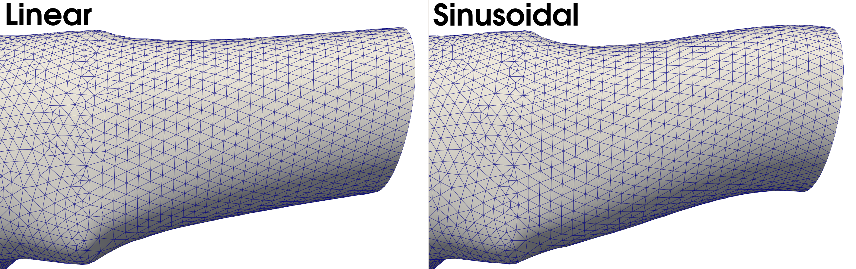
Fig. 5 On the left: A linear reduction between the image-based boundary and the end of the flow extension. On the right: A sinusiodal profile is used to gradually reduce the movement between the image-based boundary and the end of the flow extension.#
If the --clamp boundaries argument isn’t specified, the deformation at the flow extension ends will mirror the
boundary deformations observed in the image/surface-based motion.