Pre-processing

Pre-processing#

Meshing and boundary conditions#

In this brief introduction, we present VaMPy’s functionality by preparing, simulating, and post-processing models of the internal carotid artery and the left atrium, although the software may be readily used for other tubular or vascular shapes.

The first step of using the Vascular Modeling Pypeline is pre-processing. The pre-processing scripts are located inside the automatedPreprocessing folder, and can be run by using the vampy-mesh command in the terminal. The script generates a mesh, boundary conditions, and probes for velocity and pressure sampling. Here we will perform pre-processing for the artery case located in the models folder. In this example we pass the input model path (-i) and mesh coarsening factor (-c) command-line arguments:

$ vampy-mesh -i models/artery/artery.vtp -c 1.3

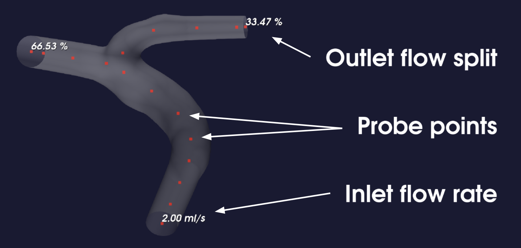
When complete, a render window will pop up showing the meshed model, prope points, flow rate and pressure split, as shown in Fig. 1. The script will save the volumetric mesh as artery.vtu, alongside a compressed DOLFIN mesh in artery.xml.gz, used for the computational fluid dynamics (CFD) simulations. The pre-processing script will also produce an info file and a probe file, named artery_info.json and artery_probes, respectively.

_images/render.png — Fig. 1 Visualization of the meshed artery model by running `vampy-mesh`.#

Dimensions and scaling#

VaMPy has been developed for models that are originally segmented from medical images, where the units are often in millimeters (mm). Hence, the current implementation assumes that the input model is in mm. It is also preferable that the model is uncapped (open), although there is some experimental methods for uncapping a surface model in case it is capped (closed).

If your input model is not in mm, you may scale it by adding the --scale-factor argument, which takes a numerical value. To scale your model from m to mm you can run the following command:

$ vampy-mesh -i models/artery/artery.vtp -c 1.3 --scale-factor 1000

Smoothing#

It may be necessary to smooth the input model in order to improve the quality of the mesh. In VaMPy, we have included three smoothing techniques that are controlled by the --smoothing-method (-sm) argument. These are Laplacian (laplace), Taubin (taubin), and Voronoi diagram smoothing (voronoi). Furthermore, for the Laplace and Taubin smoothing, the user may select the number of smoothing iterations, controlled by the --smoothing-iterations (-si) argument. Similarly, the intensity of the Voronoi diagram smoothing method may be controlled by the --smoothing-factor (-sf) argument, which ranges between 0 and 1, corresponding to 0 and 100%, respectively. By default, no smoothing is performed. To perform Laplacian smoothing using the artery model, we may run the following command:

$ vampy-mesh -i models/artery/artery.vtp -c 1.3 --smoothing-method laplace -si 800 -sf 0.75

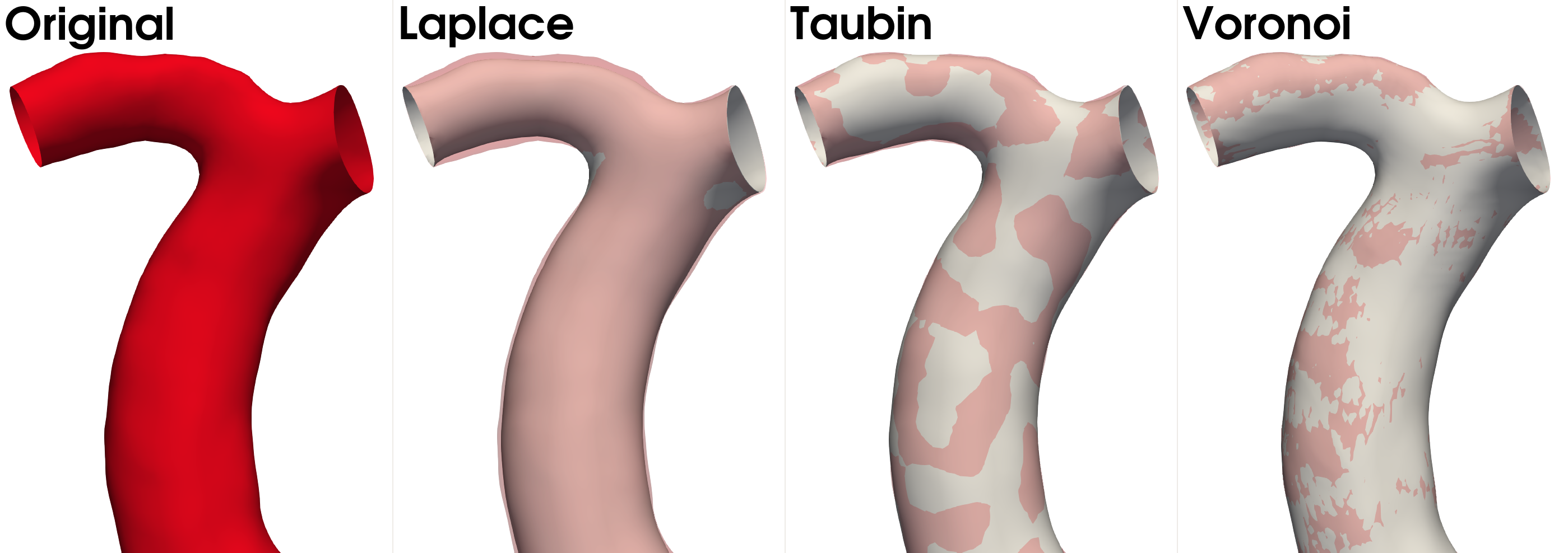
In Fig. 2, we have shown a comparison of all the smoothing methods using -si 800 and -sf 0.75, and included the original model for reference (in red).

_images/smoothing.png — Fig. 2 From left to right: the original artery model in red, and a comparison of the three smoothing methods; Laplace, Taubin and Voronoi smoothing, against the original model (red).#

Flow extensions#

Prior to mesh generation, flow extensions may be appended to the input model, often to assure that flow is fully developed as it enters and leaves the domain during CFD simulation. It is also essential to add cylindrical flow extensions when applying velocity profiles that assume a circular inlet. In VaMPy, this is controlled by the --add-flowextensions (-f) argument, which takes a boolean value and is True by default. The user may also supply the length of the flow extensions at what is considered to be the inlet(s) and outlet(s), controlled by the --inlet-flowextension (-fli) and --outlet-flowextension (-flo) command line arguments. Both are set to 5 by default, corresponding to a flow extension length equal to five times the length of the local radius at the boundary (inlet/outlet). To demonstrate, the following command will apply flow extensions to the artery model that are two and four times the local radius in length at the inlet and outlet, respectively:

$ vampy-mesh -i models/artery/artery.vtp -c 1.3 --add-flowextensions True -fli 2 -flo 4

To visualize the difference, we have shown a comparison between the original model (left) and four models with flow extensions of varying length, ranging from 1 to 4 times the local radius, in Fig. 3.

_images/flow_extension.png — Fig. 3 On the left, the original model with no flow extensions. The remining models harbor flow extensions of varying length, based on the local radius at the outlet and inlet boundary.#

Boundary layers#

In fluid flows where the Reynolds numbers are large, flow simulations will cause strong gradients near the wall, requiring fine resolution of the solution close to the boundary. In this situation it is essential to refine the finite element mesh isotropically to capture strong gradients. This is also relevant when computing hemodynamic indices on the domain boundary, such as the wall shear stress, which is demonstrated in the post-processing section. Therefore, VaMPy adds four boundary layers to the computational domain by default. However, these can be turned off by setting the --add-boundary-layer (-bl) argument to False. Thus, to skip adding boundary layers for the artery model, we may run the following command:

$ vampy-mesh -i models/artery/artery.vtp -c 1.3 --add-boundary-layer False

In Fig. 4 we demonstrate the qualitative difference when adding or removing boundary layers to the volumetric mesh.

_images/boundary_layers.png — Fig. 4 On the left, a volumetric mesh with no boundary layer. On the right, a volumetric mesh with four boundary layers, which is the default in VaMPy.#

Mething method#

There are currently three meshing methods to chose between, which determine the local mesh density. The methods are selected throught command line argument --meshing-method (-m), and can be set to either constant, diameter, or curvature. By default, the diameter method is selected. The three methods are further examined in the artery tutorial.