Post-processing

Following the CFD simulations, the last step of the Vascular Modeling Pypeline is post-processing of the results. Hemodynamic indices are computed in the script compute_hemodynamic_indices.py through the VaMPy-command vampy-hemo, and stored in a folder named Hemodynamics. Flow and simulation metrics are computed in the script compute_flow_and_simulation_metrics.py through the VaMPy-command vampy-metrics, and stored in a folder named FlowMetrics. Converting velocity and pressure to viewable .xdmf-format is performed in the script compute_velocity_and_pressure.py through the VaMPy-command vampy-convert. Finally, visualization of the velocity and pressure at the probes is implemented in visualize_probes.py and run through the vampy-probe command.

Attention

In the following examples, we assume the user is working from the root directory of VaMPy, and that the solution files produced by VaMPy (u.h5, p.h5, mesh.h5) are located inside the Solutions folder.

Hemodynamic indices

To start with we can compute the wall shear stress, oscillatory shear index (OSI) and other hemodynamic indices by executing the following command:

$ vampy-hemo --case src/vampy/simulation/results_artery/artery/data/[RUN_NUMBER]/Solutions

This produces several .xdmf and corresponding .h5 files, which can be visualized in ParaView. A list of all the computed quantities can be viewed here. In Fig. 6 we have visualized the time averaged wall shear stress ( TAWSS), temporal wall shear stress gradient (TWSSG), and relative residence time (RRT) for the artery case.

Fig. 6 Visualization of the wall shear stress (left), temporal wall shear stress gradient (middle) and the RRT (right) for the artery case. Note that all quantities have been time averaged over the last cardiac cycles.

Flow and simulation metrics

To compute fluid dynamic quantities and simulation metrics, you may execute the following command:

$ vampy-metrics --case src/vampy/simulation/results_artery/artery/data/[RUN_NUMBER]/Solutions

This produces several .xdmf and corresponding .h5 files, which can be visualized in ParaView. A list of all the computed quantities viewed here. In Fig. 7 we have visualized the kinetic energy, average velocity and the characteristic edge length for the artery model.

Fig. 7 Visualization of the time averaged kinetic energy (left), time averaged velocity (middle) and the characteristic edge length (right) for the artery case.

Velocity and pressure

For data storage reasons velocity and pressure results are currently saved in the compressed .h5 format, and are therefore not viewable in a software such as ParaView. If it is desired to convert the compressed velocity and pressure results to viewable .xdmf format, you may execute the following command:

$ vampy-convert --case src/vampy/simulation/results_artery/artery/data/[RUN_NUMBER]/Solutions

The script will store the velocity and pressure into velocity.xdmf and pressure.xdmf, respectively, to the Solutions folder. In Fig. 8 we have visualized the instanteneous veloctiy and pressure at the end of the simulation for the artery case.

Fig. 8 Visualization of the volumetric velocity (left) and scalar pressure field (right) for the artery case.

Probe visualization

To visualize velocity and pressure at the probes created by Artery.py or Atrium.py, you can run the vampy-probe command:

$ vampy-probe --case src/vampy/simulation/results_artery/artery/data/[RUN_NUMBER]/Probes --probe-frequency 100

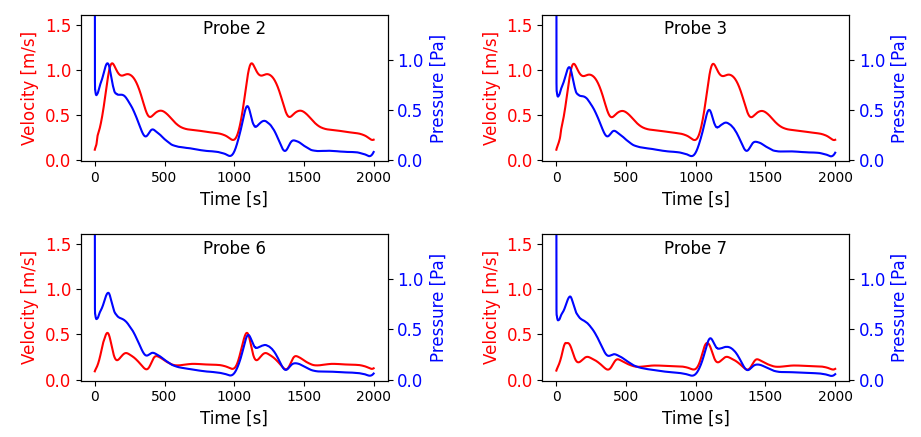
Note that you may have to adjust the --probe-frequency argument, depending on the frequency of probe sampling. The script also has an additional dependency to Matplotlib, which can easily be installed with either conda or pip. In Fig. 9 we have shown a subset of the velocity and pressure traces at four probes within the artery geometry.

Fig. 9 Probe visualization for pressure (blue) and velocity (red) at four probes within the artery geometry.

Phase and cycle averaged quantities

By default, vampy-metrics computes the average values over a full cycle, for a desired number of cycles, determined by the --start-cycle flag. Setting --start-cycle 2 would correspond to computing the averaged values from the second cardiac cycle and onward. Alternatively, the user may supply the specific times \(t\) during the cardiac cycle \(T\) to the --times-to-average flag, to compute phase averaged quantities, where \(t \in [0,T)\). To demonstrate the qualitative differences, we have simulated an open-source model of the left atrium, particularly Case 7 from Roney et al.[RBP+21] The model is simulated with Atrium.py over five cycles using \(T=951\) ms and \(\Delta t = 0.951\) ms, which are the default values in the problem file. To compute the metrics at \(t=200\Delta t\), and to skip the first cycle, run the following command:

$ vampy-metrics --case src/vampy/simulation/results_atrium/atrium/data/[RUN_NUMBER]/Solutions --start-cycle 2 --times-to-average 190.2 

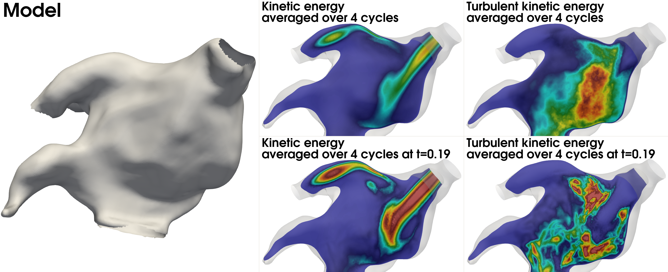
Note that the specified time (\(t=190.2\)) is in milliseconds. A comparison between time averaged and phase averaged kinetic energy (KE) and turbulent kinetic energy (TKE) for the atrium model is shown in the leftmost panel in Fig. 10. The top middle panel displays the time averaged KE over the last four cycles, whereas the bottom middle panel displays the phase averaged KE at \(t=0.19\) s. Similarly, the top right panel displays the time averaged TKE over the last four cycles, and bottom right panel displays the phase averaged TKE at \(t=0.19\) s. For this demonstration, the simulation was run over five cycles, while the metrics were computed over the last four cycles.

Fig. 10 Time and phase average kinetic energy and turbulent kinetic energy. The leftmost panel display the model, the middle panels display kinetic energy, and the rightmost panel display turbulent kinetic energy. Note that KE and TKE have been scaled independently.

Another feature of the vampy-metrics and vampy-hemo scripts is computation of time averaged quantities per cycle. This is controlled by the --average-over-cycles flag, which when supplied will output additional files that are averaged over each cycle in the format [QUANTITY]_cycle_[#CYCLE].xdmf. To demonstrate this feature, we consider the atrium model from before, and perform post-processing using the following command:

$ vampy-metrics --case src/vampy/simulation/results_atrium/atrium/data/[RUN_NUMBER]/Solutions --start-cycle 1 --average-over-cycles

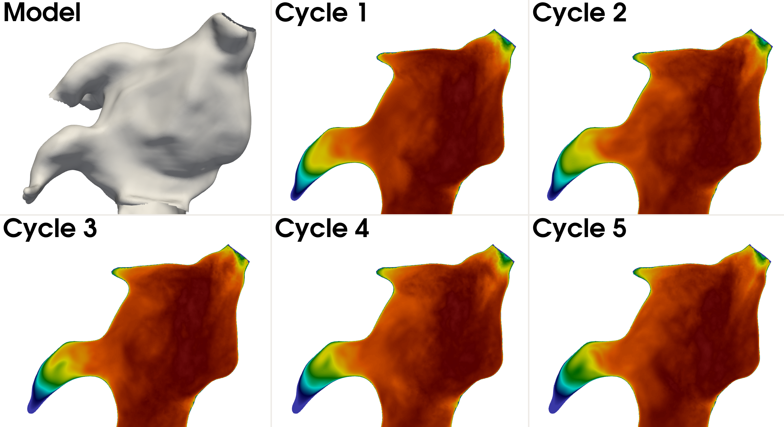
Running this command produces cycle averaged results for all the relevant quantitites. To demonstrate qualitative differences in the left atrial appendage we have shown a comparison between cycles in Fig. 10 for the TKE.

Fig. 11 Time averaged turbulent kinetic energy per cardiac cycle. The top leftmost panel display the model, and the remaining panels show a slice of the time averaged TKE for each of the cardiac cycles, showing qualitative differences in the left atrial appendage.

RBP+21

Caroline H Roney, Rokas Bendikas, Farhad Pashakhanloo, Cesare Corrado, Edward J Vigmond, Elliot R McVeigh, Natalia A Trayanova, and Steven A Niederer. Constructing a human atrial fibre atlas. Annals of biomedical engineering, 49(1):233–250, 2021.